

本部分的目标是 训练 XGBoost 票房预测模型,并进行评估与优化,确保模型具有良好的泛化能力,能够较准确地预测电影票房。
5.1 模型训练
在上一部分,我们已经选择 XGBoost Regressor 作为票房预测模型。
现在,我们使用 训练集(X_train, y_train) 进行模型训练,并评估其在测试集(X_test, y_test) 上的表现。
5.1.1 导入必要库
import xgboost as xgb
import numpy as np
import matplotlib.pyplot as plt
import seaborn as sns
from sklearn.metrics import mean_absolute_error, mean_squared_error, r2_score
from sklearn.model_selection import train_test_split, GridSearchCV, RandomizedSearchCV
5.1.2 训练 XGBoost 模型
# 初始化 XGBoost 回归模型
xgb_model = xgb.XGBRegressor(
    objective='reg:squarederror',  # 目标函数:平方误差
    n_estimators=500,  # 500 棵树
    learning_rate=0.05,  # 学习率
    max_depth=6,  # 树的最大深度
    subsample=0.8,  # 训练子样本比例
    colsample_bytree=0.8,  # 每棵树使用的特征比例
    random_state=42
)

# 训练模型
xgb_model.fit(X_train, y_train)
5.2 模型评估
训练完成后,我们使用测试集进行预测,并通过多种指标评估模型性能。
5.2.1 计算误差
# 预测测试集
y_pred = xgb_model.predict(X_test)

# 计算误差指标
mse = mean_squared_error(y_test, y_pred)
rmse = np.sqrt(mse)
mae = mean_absolute_error(y_test, y_pred)
r2 = r2_score(y_test, y_pred)

print(f"MSE: {mse:.2f}")
print(f"RMSE: {rmse:.2f}")
print(f"MAE: {mae:.2f}")
print(f"R² Score: {r2:.4f}")

# MSE: 1634638562677169.25
# RMSE: 40430663.64
# MAE: 9492384.79
# R² Score: 0.5037- MSE(均方误差):衡量预测值与真实值之间的平均平方差距。
- RMSE(均方根误差):MSE 的平方根,单位与目标变量一致。
- MAE(平均绝对误差):预测值与真实值的平均绝对偏差。
- R² 分数(决定系数):衡量模型对数据的解释能力,范围 [−∞,1],越接近 1 说明模型效果越好。
5.3 超参数优化
为了进一步提升模型表现,我们使用 网格搜索(Grid Search)和随机搜索(Randomized Search) 进行超参数调优。
5.3.1 网格搜索
网格搜索会遍历所有可能的参数组合,找到最佳参数:
param_grid = {
    'max_depth': [4, 6, 8],
    'learning_rate': [0.01, 0.05, 0.1],
    'n_estimators': [100, 300, 500],
    'subsample': [0.7, 0.8, 0.9],
    'colsample_bytree': [0.7, 0.8, 0.9]
}

grid_search = GridSearchCV(
    estimator=xgb.XGBRegressor(objective='reg:squarederror', random_state=42),
    param_grid=param_grid,
    scoring='neg_mean_squared_error',
    cv=3,
    verbose=1,
    n_jobs=-1
)

grid_search.fit(X_train, y_train)

# 获取最佳参数
best_params = grid_search.best_params_
print("Best parameters:", best_params)缺点:计算量较大,适用于小规模数据。
5.3.2 随机搜索
随机搜索相比网格搜索更高效,可以在 更大的参数空间 进行搜索:
param_dist = {
    'max_depth': np.arange(4, 10, 1),
    'learning_rate': np.linspace(0.01, 0.2, 10),
    'n_estimators': np.arange(100, 600, 100),
    'subsample': np.linspace(0.6, 1.0, 5),
    'colsample_bytree': np.linspace(0.6, 1.0, 5)
}

random_search = RandomizedSearchCV(
    estimator=xgb.XGBRegressor(objective='reg:squarederror', random_state=42),
    param_distributions=param_dist,
    n_iter=20,  # 只搜索 20 组参数
    scoring='neg_mean_squared_error',
    cv=3,
    verbose=1,
    n_jobs=-1
)

random_search.fit(X_train, y_train)

# 获取最佳参数
best_params_random = random_search.best_params_
print("Best parameters (Random Search):", best_params_random)优点:可以在更大参数空间进行搜索,计算量较小。
5.4 训练最终优化模型
使用最佳参数重新训练模型:
# 使用最优参数训练 XGBoost
xgb_final = xgb.XGBRegressor(
    **best_params_random,  # 使用随机搜索的最优参数
    objective='reg:squarederror',
    random_state=42
)

xgb_final.fit(X_train, y_train)

# 预测测试集
y_pred_final = xgb_final.predict(X_test)

# 计算最终误差
mse_final = mean_squared_error(y_test, y_pred_final)
rmse_final = np.sqrt(mse_final)
mae_final = mean_absolute_error(y_test, y_pred_final)
r2_final = r2_score(y_test, y_pred_final)

print(f"Final MSE: {mse_final:.2f}")
print(f"Final RMSE: {rmse_final:.2f}")
print(f"Final MAE: {mae_final:.2f}")
print(f"Final R² Score: {r2_final:.4f}")


# Final MSE: 1269856550614248.25
# Final RMSE: 35635046.66
# Final MAE: 9145602.70
# Final R² Score: 0.6145
如果 R² 分数提高、RMSE 降低,说明调优成功。
5.5 结果可视化
为了更直观地评估模型,我们绘制一些可视化图表。
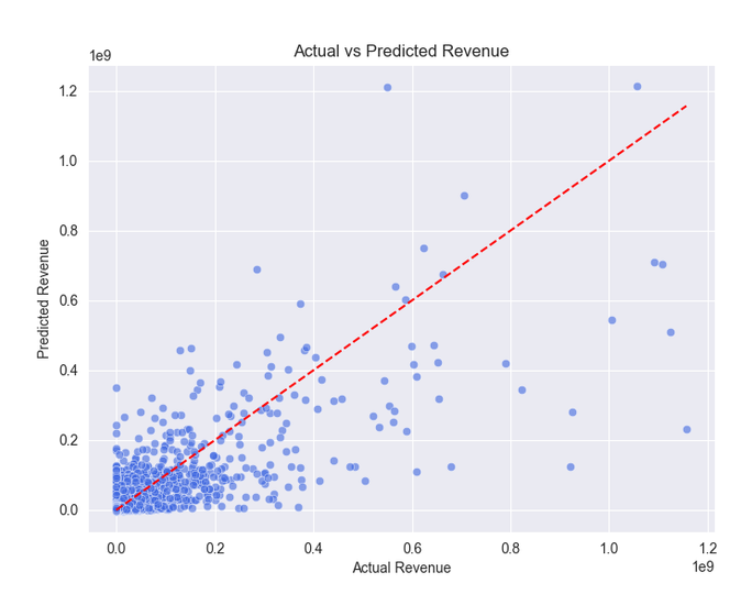
5.5.1 真实值 vs 预测值
plt.figure(figsize=(8, 6))
sns.scatterplot(x=y_test, y=y_pred_final, alpha=0.6, color="royalblue")
plt.plot([min(y_test), max(y_test)], [min(y_test), max(y_test)], linestyle="--", color="red")  # 参考线
plt.xlabel("Actual Revenue")
plt.ylabel("Predicted Revenue")
plt.title("Actual vs Predicted Revenue")
plt.show()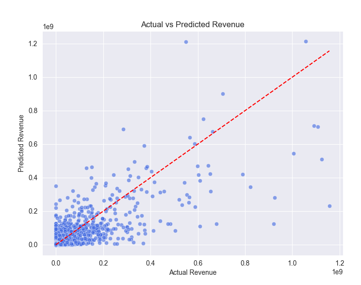
红色虚线 代表理想预测,点越接近该线说明预测越准确。
5.5.2 误差分布
plt.figure(figsize=(8, 6))
sns.histplot(y_test - y_pred_final, bins=30, kde=True, color="orange")
plt.xlabel("Prediction Error")
plt.ylabel("Frequency")
plt.title("Prediction Error Distribution")
plt.show()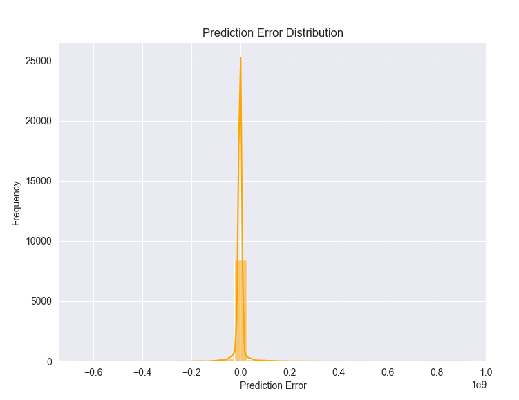
如果误差分布呈 正态分布且均值接近 0,说明模型误差较小。
5.6 小结
- 训练 XGBoost 模型,初步评估其在测试集上的误差。
- 使用网格搜索和随机搜索,优化超参数,提升预测精度。
- 训练最终优化模型,并评估其误差降低情况。
- 使用可视化技术分析结果,包括预测误差分布、真实 vs 预测值对比。
© 版权声明
文章版权归作者所有,未经允许请勿转载。
THE END











请登录后查看评论内容