

在这一阶段,我们将实现模型的训练,使用适当的评价指标对模型性能进行评估,并通过网格搜索或随机搜索优化模型的超参数。最后,我们将选择合适的可视化形式,展示模型评估结果。
5.1 模型训练
首先,我们将使用前面选择的 XGBoost 模型进行训练。
from xgboost import XGBClassifier
from sklearn.metrics import classification_report, confusion_matrix, roc_auc_score, accuracy_score
from sklearn.model_selection import GridSearchCV

# 构建并训练XGBoost分类器
xgb_model = XGBClassifier(
    n_estimators=100,  # 初始树数量
    learning_rate=0.1,  # 初始学习率
    max_depth=4,  # 树的最大深度
    scale_pos_weight=3,  # 处理类别不平衡问题
    random_state=42  # 固定随机数种子
)

# 训练模型
xgb_model.fit(X_train, y_train)

# 测试集预测
y_pred = xgb_model.predict(X_test)
5.2 模型评估
为了全面评估模型的性能,我们将使用以下指标:
- 准确率(Accuracy):预测正确的样本占总样本的比例。
- 精确率(Precision):被预测为流失客户的样本中,实际为流失客户的比例。
- 召回率(Recall):实际流失的客户中,模型能正确预测的比例。
- F1 分数:精确率和召回率的调和平均数,综合评估模型性能。
- AUC-ROC 曲线:评估模型的二元分类性能,AUC 值越接近1,表示模型效果越好。
# 输出混淆矩阵、分类报告和AUC值
print(confusion_matrix(y_test, y_pred))
print(classification_report(y_test, y_pred))

# 计算AUC分数
y_pred_prob = xgb_model.predict_proba(X_test)[:, 1]  # 获取流失客户的预测概率
auc = roc_auc_score(y_test, y_pred_prob)
print(f"AUC Score: {auc:.2f}")
5.3 模型优化(超参数调优)
为了进一步提升模型性能,我们将使用 网格搜索(Grid Search) 进行超参数调优。
常见的超参数包括 n_estimators、max_depth、learning_rate 和 scale_pos_weight。
通过遍历不同的超参数组合,找到性能最优的模型。
# 定义超参数网格
param_grid = {
    'n_estimators': [100, 200],
    'max_depth': [3, 4, 5],
    'learning_rate': [0.01, 0.1, 0.2],
    'scale_pos_weight': [1, 2, 3]
}

# 网格搜索
grid_search = GridSearchCV(estimator=XGBClassifier(random_state=42),
                           param_grid=param_grid,
                           scoring='roc_auc',
                           cv=3,
                           verbose=1)

# 训练网格搜索模型
grid_search.fit(X_train, y_train)

# 输出最佳参数
print("Best parameters found: ", grid_search.best_params_)

# 使用最佳参数训练最终模型
best_xgb_model = grid_search.best_estimator_
y_best_pred = best_xgb_model.predict(X_test)

# 输出最佳模型的评估结果
print(classification_report(y_test, y_best_pred))
5.4 模型评估结果可视化
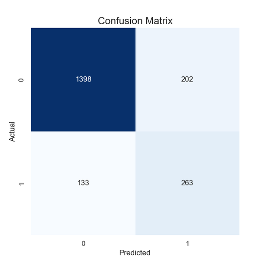
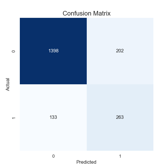
我们将通过绘制 混淆矩阵 和ROC-AUC 曲线 直观地展示模型的性能~
# 导入绘图库
import matplotlib.pyplot as plt
import seaborn as sns
from sklearn.metrics import roc_curve, confusion_matrix

# 绘制混淆矩阵
def plot_confusion_matrix(y_true, y_pred):
    cm = confusion_matrix(y_true, y_pred)
    plt.figure(figsize=(6, 6))
    sns.heatmap(cm, annot=True, fmt="d", cmap="Blues", cbar=False)
    plt.title("Confusion Matrix", fontsize=16)
    plt.ylabel('Actual', fontsize=12)
    plt.xlabel('Predicted', fontsize=12)
    plt.show()

# 绘制ROC曲线
def plot_roc_curve(y_true, y_pred_prob):
    fpr, tpr, thresholds = roc_curve(y_true, y_pred_prob)
    plt.figure(figsize=(8, 6))
    plt.plot(fpr, tpr, color="orange", label=f'AUC = {auc:.2f}')
    plt.plot([0, 1], [0, 1], linestyle='--', color='gray')
    plt.title("ROC Curve", fontsize=16)
    plt.xlabel("False Positive Rate", fontsize=12)
    plt.ylabel("True Positive Rate", fontsize=12)
    plt.legend(loc="lower right")
    plt.grid(True)
    plt.show()

# 绘制混淆矩阵和ROC曲线
plot_confusion_matrix(y_test, y_best_pred)
plot_roc_curve(y_test, best_xgb_model.predict_proba(X_test)[:, 1])
5.5 评价总结
我们使用了以下评价指标对模型进行评估:
- 混淆矩阵:展示了模型的分类情况,包括 TP(真正例)、TN(真负例)、FP(假正例)和 FN(假负例)。
- 分类报告:输出了精确率、召回率和 F1 分数,综合评估模型的分类性能。
AUC-ROC 曲线:展示了模型的 AUC 值,以评估其二元分类的效果。
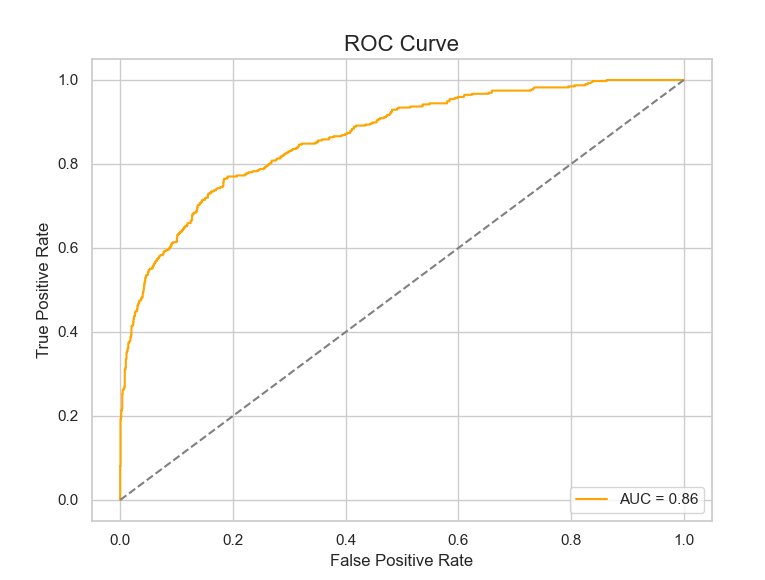
通过可视化展示,我们能够直观地看到模型的分类能力和区分流失客户的能力。
5.6 小结
- 模型训练:我们使用了XGBoost模型进行了客户流失预测的训练。
- 模型评估:通过混淆矩阵、精确率、召回率、F1分数和AUC值全面评估了模型的性能。
- 超参数调优:通过网格搜索优化了超参数,找到了最优的参数组合,进一步提升了模型性能。
- 可视化展示:通过混淆矩阵和ROC-AUC曲线直观地展示了模型的分类性能,提升了分析的可解释性。
6. 结果分析与解读
© 版权声明
文章版权归作者所有,未经允许请勿转载。
THE END











请登录后查看评论内容