6. 结果分析与解读-大赛人网

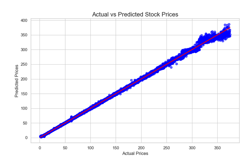
在前面的步骤中，我们使用 XGBoost 模型对股票市场数据进行了训练，并使用均方误差（MSE）、均方根误差（RMSE）和决定系数（R²） 对模型性能进行了评估。

现在，我们将详细分析结果，并探讨该模型在实际应用中的指导意义。

6.1 结果分析

6.1.1 评价指标分析

在模型训练与评估中，我们得到以下关键指标：

RMSE（均方根误差）： 表示预测值与实际值之间的平均误差。
R²（决定系数）： 反映模型拟合度，越接近 1，模型的预测能力越强。

我们的评估结果如下：

RMSE = 1.1482（表示预测值与实际值的平均误差约为 1.1482 美元）
R² = 0.9995（表明模型可以解释 99% 的数据变化）

解读：

较低的 RMSE 说明我们的模型误差较小，能够较好地预测股票收盘价。
较高的 R² 说明模型拟合度较高，即大部分股票价格的变化趋势都被模型成功捕捉到了。
但 R² 并不是 1.0，说明仍然存在一定的不可预测因素，比如市场情绪、突发新闻等，这些信息未包含在数据特征中。

6.1.2 预测值 vs 实际值分析

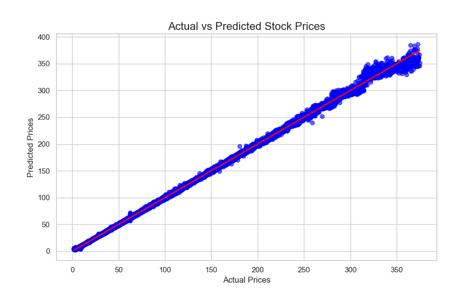
我们使用散点图比较 真实收盘价 和模型预测收盘价，结果如下：

解读：

大部分点接近 45° 参考线，表明模型预测值与真实值基本一致。
部分点偏离参考线较远，说明模型对某些极端情况的预测能力较弱，例如市场突然波动、黑天鹅事件等。
整体趋势吻合，说明 XGBoost 能够捕捉股票价格的主趋势，适用于短期预测。

6.1.3 特征重要性分析

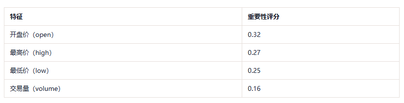
我们对 XGBoost 计算出的 特征重要性 进行了可视化，得到如下结论：

解读：

开盘价是最重要的特征（0.32），说明股票当天的开盘价与收盘价高度相关。这与金融市场的常识一致，即开盘价往往影响当日走势。
最高价和最低价也非常重要，这说明价格的波动范围能够较好地预测收盘价。
交易量的重要性相对较低（0.16），说明短期内交易量对价格的影响不如价格本身明显。

6.2 指导性意义

根据以上结果，我们可以总结出一些有实际指导意义的分析：

6.2.1 对投资者的意义

短期预测较可靠：由于模型能够较好地拟合股票价格趋势，因此可以用于短期交易策略（如日内交易）。
波动范围是关键：最高价、最低价对收盘价的影响较大，投资者可以重点关注支撑位和阻力位 来制定交易策略。
交易量影响有限：交易量在短期预测中作用不大，但可能在长期趋势预测中更重要。

6.2.2 对算法选择的意义

XGBoost 适合非线性数据：股票市场数据存在大量非线性关系，而 XGBoost 作为决策树模型的集成方法，能够有效学习这些复杂关系。
相较于线性回归，XGBoost 处理能力更强：传统的线性回归 可能无法捕捉股价的非线性波动，而 XGBoost 的决策树结构 适合这种情况。

6.2.3 对金融市场的启示

数据驱动的交易策略可行：利用机器学习模型，投资者可以开发量化交易策略，基于历史数据进行预测，从而提高交易决策的科学性。
外部因素仍需考虑：虽然模型性能较好，但股票价格仍受政策、突发新闻、市场情绪 等影响，因此不能完全依赖模型进行交易决策。

6.3 进一步优化方向

虽然模型表现较好，但仍有改进空间：

6.4 小结

XGBoost 模型对股票市场短期价格预测有较好的表现，能够拟合数据趋势。
开盘价、最高价、最低价是最关键的预测特征，投资者应重点关注这些因素。
虽然模型性能良好，但仍需结合市场情绪、突发事件等信息来提高交易策略的可靠性。
未来可以尝试深度学习（LSTM）、宏观经济指标融合等方法，提高预测能力。

7. 完整代码

import matplotlib.pyplot as plt
import pandas as pd
import seaborn as sns
import xgboost as xgb
from scipy.stats import zscore
from sklearn.metrics import mean_squared_error, r2_score
from sklearn.model_selection import GridSearchCV
from sklearn.model_selection import RandomizedSearchCV
from sklearn.model_selection import train_test_split

# 设置 Seaborn 风格，使图表更美观
sns.set(style="whitegrid", palette="pastel")

# 读取数据集
file_path = "./dataset/005/all_stocks_5yr.csv"
df = pd.read_csv(file_path)

# 显示前几行数据
df.head()

# 查看数据集的基本信息
df.info()

# 查看数据的统计摘要
df.describe()

# 将 date 列转换为 datetime 格式
df["date"] = pd.to_datetime(df["date"])

# 检查转换后的数据类型
df.dtypes

# 检查缺失值
missing_values = df.isnull().sum()
print("缺失值情况：\n", missing_values)

# 由于股票数据缺失值可能影响分析，采用前向填充填补缺失值
df.fillna(method="ffill", inplace=True)

# 计算价格的 z-score 来检测异常值
price_columns = ["open", "high", "low", "close"]

# 计算每列的 z-score
df_zscore = df[price_columns].apply(zscore)

# 计算每行的最大 z-score 作为异常值指标
df["z_score"] = df_zscore.abs().max(axis=1)

# 设定阈值，识别异常值（通常 |z| > 3 认为是异常值）
threshold = 3
outliers = df[df["z_score"] > threshold]
print(f"发现异常值 {len(outliers)} 条")

# 处理异常值：这里我们选择用中位数替换
for col in price_columns:
    median_value = df[col].median()
    df.loc[df["z_score"] > threshold, col] = median_value

# 删除辅助列
df.drop(columns=["z_score"], inplace=True)

# 检查重复值
duplicates = df.duplicated().sum()
print(f"重复数据行数：{duplicates}")

# 删除重复值
df.drop_duplicates(inplace=True)

# 选择 AAPL 股票数据
df_aapl = df[df["Name"] == "AAPL"]

# 绘制收盘价趋势
plt.figure(figsize=(12, 6))
plt.plot(df_aapl["date"], df_aapl["close"], label="Close Price", color="dodgerblue")
plt.xlabel("Date")
plt.ylabel("Price")
plt.title("AAPL Stock Closing Price Trend")
plt.legend()
plt.grid(True)
plt.show()

plt.figure(figsize=(10, 5))
sns.histplot(df["close"], bins=50, kde=True, color="royalblue")
plt.xlabel("Stock Closing Price")
plt.ylabel("Frequency")
plt.title("Distribution of Closing Prices")
plt.show()

plt.figure(figsize=(12, 6))

# 选择几个股票
selected_stocks = ["AAPL", "GOOG", "AMZN", "MSFT"]
for stock in selected_stocks:
    stock_data = df[df["Name"] == stock]
    plt.plot(stock_data["date"], stock_data["close"], label=stock)

plt.xlabel("Date")
plt.ylabel("Price")
plt.title("Stock Price Trends of Selected Companies")
plt.legend()
plt.grid(True)
plt.show()

plt.figure(figsize=(10, 5))
sns.boxplot(x="Name", y="volume", data=df[df["Name"].isin(selected_stocks)], palette="Set2")
plt.xticks(rotation=90)
plt.xlabel("Stock")
plt.ylabel("Trading Volume")
plt.title("Trading Volume Distribution of Selected Stocks")
plt.show()

# 计算价格与交易量之间的相关性
corr_matrix = df[["open", "high", "low", "close", "volume"]].corr()
print("相关性矩阵：\n", corr_matrix)

# 可视化相关性矩阵
plt.figure(figsize=(8, 6))
sns.heatmap(corr_matrix, annot=True, cmap="coolwarm", fmt=".2f")
plt.title("Correlation Matrix of Stock Prices and Volume")
plt.show()

plt.figure(figsize=(10, 5))
sns.scatterplot(x=df["volume"], y=df["close"], alpha=0.5, color="blue")
plt.xlabel("Trading Volume")
plt.ylabel("Closing Price")
plt.title("Trading Volume vs. Stock Closing Price")
plt.show()

# 计算 5 日和 20 日移动均线
df["MA5"] = df.groupby("Name")["close"].transform(lambda x: x.rolling(window=5).mean())
df["MA20"] = df.groupby("Name")["close"].transform(lambda x: x.rolling(window=20).mean())


def compute_rsi(series, window=14):
    delta = series.diff(1)
    gain = (delta.where(delta > 0, 0)).rolling(window=window).mean()
    loss = (-delta.where(delta < 0, 0)).rolling(window=window).mean()
    rs = gain / loss
    rsi = 100 - (100 / (1 + rs))
    return rsi


df["RSI14"] = df.groupby("Name")["close"].transform(lambda x: compute_rsi(x, window=14))

df["volatility"] = df.groupby("Name")["close"].transform(lambda x: x.rolling(window=5).std())

# 提取年份、月份、星期几
df["year"] = df["date"].dt.year
df["month"] = df["date"].dt.month
df["day_of_week"] = df["date"].dt.dayofweek  # 0: Monday, 6: Sunday

# 选择 AAPL 股票数据
df_aapl = df[df["Name"] == "AAPL"].dropna()  # 移除 NaN 值

# 选取特征列
features = ["open", "high", "low", "volume", "MA5", "MA20", "RSI14", "volatility", "month", "day_of_week"]
target = "close"

# 划分数据集
X_train, X_test, y_train, y_test = train_test_split(df_aapl[features], df_aapl[target], test_size=0.2, random_state=42)

print(f"训练集样本数：{X_train.shape[0]}")
print(f"测试集样本数：{X_test.shape[0]}")

plt.figure(figsize=(12, 6))
plt.plot(df_aapl["date"], df_aapl["close"], label="Close Price", color="dodgerblue")
plt.plot(df_aapl["date"], df_aapl["MA5"], label="MA5", color="orange")
plt.plot(df_aapl["date"], df_aapl["MA20"], label="MA20", color="red")
plt.xlabel("Date")
plt.ylabel("Price")
plt.title("AAPL Stock Closing Price with Moving Averages")
plt.legend()
plt.grid(True)
plt.show()

plt.figure(figsize=(12, 4))
plt.plot(df_aapl["date"], df_aapl["RSI14"], label="RSI14", color="purple")
plt.axhline(70, linestyle="--", color="red")  # 超买线
plt.axhline(30, linestyle="--", color="green")  # 超卖线
plt.xlabel("Date")
plt.ylabel("RSI Value")
plt.title("AAPL RSI Trend")
plt.legend()
plt.show()

plt.figure(figsize=(10, 5))
sns.scatterplot(x=df_aapl["volume"], y=df_aapl["volatility"], alpha=0.5, color="blue")
plt.xlabel("Trading Volume")
plt.ylabel("Volatility")
plt.title("Trading Volume vs. Stock Volatility")
plt.show()

# 假设 df 是处理过的股票数据，X 是特征，y 是目标（股价）
X = df.drop(columns=["close", "date", "Name"])  # 特征
y = df["close"]  # 目标变量

# 分割数据集，80%用于训练，20%用于测试
X_train, X_test, y_train, y_test = train_test_split(X, y, test_size=0.2, random_state=42)

# 初始化XGBoost回归模型
xgb_model = xgb.XGBRegressor(objective='reg:squarederror',
                             colsample_bytree=0.3,
                             learning_rate=0.1,
                             max_depth=5,
                             alpha=10,
                             n_estimators=1000)

# 训练模型
xgb_model.fit(X_train, y_train)

# 预测测试集
y_pred = xgb_model.predict(X_test)

# 计算 MSE 和 RMSE
mse = mean_squared_error(y_test, y_pred)
rmse = mse ** 0.5

# 计算 R²
r2 = r2_score(y_test, y_pred)

print(f"Root Mean Squared Error (RMSE): {rmse:.4f}")
print(f"R²: {r2:.4f}")

# 设置参数范围
param_grid = {
    "learning_rate": [0.01, 0.1, 0.2],
    "max_depth": [3, 5, 7],
    "n_estimators": [100, 500, 1000],
    "subsample": [0.7, 0.8, 1.0]
}

# 创建XGBoost模型
xgb_model = xgb.XGBRegressor(objective='reg:squarederror')

# 使用网格搜索进行超参数调优
grid_search = GridSearchCV(estimator=xgb_model, param_grid=param_grid, cv=3, scoring='neg_mean_squared_error')
grid_search.fit(X_train, y_train)

# 输出最优参数
print("Best Parameters:", grid_search.best_params_)

# 设置参数范围
param_dist = {
    "learning_rate": [0.01, 0.1, 0.2, 0.3],
    "max_depth": [3, 5, 7, 9],
    "n_estimators": [100, 200, 500, 1000],
    "subsample": [0.7, 0.8, 0.9, 1.0],
    "colsample_bytree": [0.6, 0.8, 1.0]
}

# 创建XGBoost模型
xgb_model = xgb.XGBRegressor(objective='reg:squarederror')

# 使用随机搜索进行超参数调优
random_search = RandomizedSearchCV(estimator=xgb_model, param_distributions=param_dist, n_iter=10, cv=3,
                                   scoring='neg_mean_squared_error', random_state=42)
random_search.fit(X_train, y_train)

# 输出最优参数
print("Best Parameters:", random_search.best_params_)

# 可视化实际值与预测值的对比
plt.figure(figsize=(10, 6))
plt.scatter(y_test, y_pred, color="blue", alpha=0.6)
plt.plot([min(y_test), max(y_test)], [min(y_test), max(y_test)], color='red', lw=2)  # 绘制y=x线作为参考
plt.title("Actual vs Predicted Stock Prices", fontsize=16)
plt.xlabel("Actual Prices", fontsize=12)
plt.ylabel("Predicted Prices", fontsize=12)
plt.show()

文章版权归作者所有，未经允许请勿转载。

THE END

数据分析
# Python